picard-lindelof

This is the first part in a series about theorems in analysis. Specifically, they are biased towards functional analysis, just as a coincidence. These theorems are ones that might be mentioned, but not typically covered in detail, in a first real analysis course. However, each are interesting in their own right. This section will be updated with each entry's respective links as I add more to the list.

Despite all of these topics being focused on concepts and strategies from analysis, I write about them as informally as possible and don't assume that you have taken a real analysis course. I assume you've taken, or are familiar with, some concepts from high-school calculus, but none of the entries will solely consist of computation, instead focusing as much as possible on telling a story, whatever that might mean.

I tried to strike a balance between broader accessibility and technical detail, but didn't want to inundate the reader with a bunch of prerequisite definitions and theorems up front. (So, regretfully, things like closed & open sets, continuity, and supremum won't be defined here.)

The big picture of the proof of Picard-Lindelof is given in the first few paragraphs under the proof heading, before Now comes the real legwork. I would like for any interested reader to take away at least that much from this exposition, as it is by far the most satisfying and aesthetically pleasing part of the proof—the meat of it, you could say.

If you spot any errors, contact me here.

entries

1. Picard-Lindelof: you're here.
2. Riemann-Lebesgue & Fourier series
3. Stone-Weierstrass
4. Arzelà-Ascoli
5. Peano existence
6. Hahn-Banach

prototype: initial value problem

You might have seen an equation like this before in Calculus II, if you've taken it. Maybe you've taken a standalone differential equations class, in which case you've definitely seen this before.

What is special about this kind of equation is that the unknown is a function \( x(t) \), not a number. Such an equation is, as expected, called a functional equation. Just like with equations involving numbers, when considering functional equations, we have to consider the existence and uniqueness of a potential solution.

The general solution to the above IVP (initial value problem) is, as you might know, the exponential function \( f(x) = Ce^{x} \). It is a calculus fact that the derivative of the exponential function is just the exponential itself. So a priori, we've found a solution.

But this isn't very clarifying or satisfying, since it seems like we were just lucky to happen to have a function whose derivative is itself. What about arbitrary initial-value problems, such as ones that deal with higher-order derivatives, or more complicated expressions on the right-hand side? What guarantees that a solution has to exist, anyways? And that such a solution has to be unique?

In Calculus II, we take it for granted that for whatever IVP you are given, there must be a solution that you can compute by hand. In a first differential equations class, the problem of existence and uniqueness is broached, but probably not belabored and proved in full detail.

banach fixed-point theorem

I've mentioned a fixed-point theorem (Brouwer's) in a previous post, but it turns out that there are a lot of them in analysis and topology, and they are all quite useful. The one we are going to use is called the contraction mapping theorem, or Banach fixed-point theorem.

First, we will define a contraction. A continuous map \( f : [a,b] \rightarrow [a,b] \) is a contraction if there exists some \( 0 \le K < 1 \) such that for any pair \( x, y \) in \( [a,b] \), \[ \lvert f(x) - f(y) \rvert \le K\lvert x - y \rvert. \] Intuitively, this means that if you have two points \( x \) and \( y \) on the number line and plug them into the function \( f \), the distance between \( f(x) \) and \( f(y) \) is always less than or equal to the distance between \( x \) and \( y \), so the map pushes everything closer together.

The Banach fixed point theorem states that if \( A \) is some non-empty, closed subset of the real line with a contraction mapping \( K : A \rightarrow A \), then \( K \) admits a unique fixed point \( x^{\ast} \) in \( A \). Further, you can find \( x^{\ast} \) by picking any \( x_{0} \) in \( A \) and defining a sequence \( x_{n} = T(x_{n-1}) \) for \( n \) a positive integer. Then \( x^{\ast} = \lim_{n \rightarrow \infty} x_{n} \), i.e., what happens when you apply the contraction a very large number of times.

I like this theorem because it is intuitive, and its statement gives a roadmap to how you could prove it. We won't prove it here, but it relies on the fact that \( A \) should be complete and that all Cauchy sequences (sequences whose terms get arbitrarily close together) converge in a complete space. Like Brouwer's fixed point theorem, which has the visual of stirring sugar into a coffee cup, Banach's theorem too has a nice, tactile sort of intuition: if you have a mapping from a set to itself which pulls everything closer together, and you iterate that mapping, eventually you will have squeezed everything down to a single point.

I introduced the Banach theorem in the context of the real line \( \mathbb R \), but it works for any metric space. A metric space is a set equipped with a binary function to the non-negative real numbers, with certain properties. They are called positive-definiteness (or non-degeneracy), symmetry, and the triangle inequality. You can read more about their definitions on the Wikipedia page for metric space. This function is called a metric, or distance, since it takes in any pair of elements from the set and spits out the distance between them. On the real line, the usual (Euclidean) distance is expressed \[ d(x,y) = \lvert x - y \rvert, \] where \( x \) and \( y \) are any pair of real numbers.

In two dimensions, the Euclidean distance may be familiar from your knowledge of the Pythagorean theorem: the square root of the sum of the squared distance between every component: \[ d(\mathbf x, \mathbf y) = \sqrt{\sum_{i=1}^2 \lvert x_i - y_i \rvert^2}. \]

In order to be able to apply the Banach fixed-point theorem to the IVP existence & uniqueness problem, we need to have a complete (and non-empty) metric space, and this metric space has to have elements that are functions. For this theorem, we will use the space of multivariate continuous functions on a compact domain \( D \subset \mathbb R \times \mathbb R^{n} \), written \( C(D, R^{n+1}) \), equipped with the \( \sup \) metric. Sometimes authors will call this the metric induced by the \( \sup \) norm or the uniform norm, but the point is that this is a very common metric used in analysis, and in general for any compact set \( K \), \( C(K) \), the set of continuous functions with compact support \( K \), is a complete metric space. (In fact, it's more than that, as we will mention promptly.) In fact, if the author does not explicitly mention what metric they are using, you can often assume that it is the \( \sup \) metric. It is also denoted \( \lVert f - g \rVert \) or \( \lVert f - g \rVert_\infty \). I'm pretty sure the \( \infty \) refers to the \( L_\infty \) norm notation from \( L_p \) spaces.

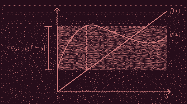
Returning to our metric space, for any two functions \( f,g \) in \( C(D, \mathbb R^{n+1}) \), the distance between them is defined \[ d(f,g) := \sup_{(t,x) \in D} \lvert f(x) - g(x) \rvert. \] In prose, the distance between \( f \) and \( g \) on a domain \( D \) is the absolute value of the maximum difference between \( f \) and \( g \) evaluated at a particular \( x \) in \( D \), visualised in the simple 2-dimensional case in Fig 2:

We will not prove here that this is indeed a metric space, but it isn't too hard to show. To see that it is a complete metric space (i.e., a Banach space, which is really a complete normed vector space Generally, vectors are things we can scale (by multiplying by some constant) and add together. This is called taking linear combinations of vectors. In our case, our vectors are continuous functions with a shared compact domain. Our field of scalars is the real numbers, \( \mathbb R \). ) isn't obvious. Its completeness comes from the fact that a sequence of functions \( x_n(t) \), for a fixed \( t \), converges uniformly to some \( x(t) \), and that the uniform limit of a sequence of continuous functions is again continuous. But for now, let's just run with it.

Moving forward, we will be referring to a more general IVP than what was shown at the beginning of this entry. It looks like:

where we will have some restrictions on \( f \) and the use of \( t_0 \) just reflects the fact that our initial time does not necessarily have to be \( t = 0 \).

picard-lindelof theorem

Now we are prepared for the Picard-Lindelof theorem.

hypotheses

\( f : D \rightarrow \mathbb R \) must be in \( C(D, \mathbb R \times \mathbb R^{n}) \) where \( D \) is some closed rectangle Picard-Lindelof actually holds for more general domains, not just closed rectangles, but the closed rectangle version is given here as a simplification. in \( \mathbb R^{n+1} \). Our initial condition \( t_{0}, x_{0} \) must be in the interior of \( D \), so not on the "borders" of the rectangle. \( f \) must be uniformly continuous in \( t \) and Lipschitz continuous in \( x \).

conclusion

There exists some \( \varepsilon > 0 \) such that there is a unique solution \( x \) to the IVP \( x'(t) = f(t,x(t)) \) with initial condition \( x(t_{0}) = x_{0} \), in \( (t_{0} - \varepsilon, t_{0} + \varepsilon) \). It is possible to more specifically characterise the maximal interval of where a solution exists, and you can derive this maximal interval by proving Peano's theorem.

The Picard-Lindelof theorem asserts the existence and uniqueness of a solution to the IVP, but it doesn't necessarily tell us what the solution looks like. Fortunately, in the process of proving Picard-Lindelof, there is a pretty natural explanation of how to (sometimes, maybe, if you're lucky) get to a concrete solution.

proof

First we assert that \( x \) being a solution of the IVP is equivalent to \( x \) solving the below integral equation:

This chain of equalities results from taking the integral on both sides of our IVP. In particular, this follows from the Fundamental Theorem of Calculus and an algebraic manipulation. Now, for very small values of \( t \), we can approximate \( x \) with \( x_{0} \). Plugging it in, we get

and repeating this process, we get

This is called Picard iteration It might be tempting to think that Picard iteration gives us a deterministic cookbook recipe on how to solve any IVP that fulfills the hypotheses of Picard-Lindelof, or at least guarantee us a good-enough approximate solution. However, it is not computationally practical to solve for arbitrary integrals. This is just fine, though, because we are mainly interested in the fact that a solution exists at all (and that it is unique), not in what exactly the solution is. and the crux of the proof of Picard-Lindelof is showing that this integral operator is a contraction mapping, and thus by application of Banach, admits a unique fixed point \( x \), which is our solution, i.e.,

is our solution.

Now comes the real legwork. Assume that \( t_0 = 0 \) as a simplification. Since \( (t_0,x_0) \) is in the interior of \( D \), we are free to choose a closed ball of radius \( \delta > 0 \) around \( x_0 \), i.e., the interval \( \overline{B_\delta(x_0)} = [x_0 - \delta, x_0 + \delta ] \). We will consider the closed interval \( [0,T] \) for \( t_0 \) where \( T \) is some suitable positive constant.

Denote \( K = [0,T] \times \overline{B_\delta(x_0)} \). In particular, \( B = \overline{B_\delta(x_0)} \) will be our closed subset of our Banach space to which we can apply Banach's theorem. Now we will define the Picard operator \[ \Gamma(x)(t) := x_0 + \int_{t_0}^t f(s,x(s)) ds, \] where \( t \) is in \( [0, T] \) (recall that we set \( t_0 = 0 \)), and we will show that \( \Gamma \) takes \( B \) to itself.

To show this, let \( x \) be an arbitrary element of \( B \). We wish to show that \[ \lvert x(t) - x_0 \rvert < \delta \implies \lvert \Gamma (x)(t) - x_0 \rvert < \delta. \]

Writing it out, we see that \[ \lvert \Gamma (x)(t) - x_0 \rvert = \left\lvert \int_{0}^t f(s,x(s)) ds \right\rvert. \]

This suggests that we should try to bound Once, a classmate remarked that analysis is all about bullying numbers to get into convenient bounds, and I think about it every time I see a bound in an analysis proof, which is every time I see an analysis proof... the right-hand side of the above somehow. One useful bound is \[ M = \sup_{(t,x) \in K}\lvert f(t,x) \rvert \] where \( M \) exists It is an analysis fact that a continuous function with compact support attains its minimum and maximum. This is the extreme value theorem. because \( K \) is compact (it is the Cartesian product of two compact sets) and because \( f \) is continuous. Then we have \[ \lvert \Gamma (x)(t) - x_0 \rvert \le \left\lvert \int_{0}^t f(s,x(s)) ds \right\rvert \le \int_{0}^t \left\lvert f(s,x(s)) \right\rvert ds \le tM, \] whenever \( (t,x(t)) \) is in \( K \). So let \( T_0 = \min \left\{ T, \frac{\delta}{M} \right\} \) and consider the interval \( [0,T_0] \). We see that \( [0,T_0] \subseteq [0,T] \), with equality attained when \( M = 0 \). But more important, since \( [0,T_0] \) is contained inside \( [0,T] \), the same constant \( M \) will also work as an upper bound for \( \lvert f \rvert \) on \( K_0 = [0,T_0] \times \overline{B_\delta(x_0)} \subseteq K \).

In summary, by choosing the values of \( t \) carefully (in specific, \( t \) must be less than \( T_0 \)), we can ensure that \( \Gamma \) is a map that takes \( B \) to itself.

Now all that is left to do is show that \( \Gamma \) is a contraction. To do so, we wish to bound

Here is where the rest of our hypotheses kick in. Recall that we required \( f \) to be Lipschitz continuous in the second argument, \( x(t) \). We actually do not require global Lipschitz continuity, only local. A function \( f \) is locally Lipschitz continuous if for every compact set of its domain, there exists a nonnegative real \( L\) such that

where \( x, y \) are in the compact set. So in our case, since \( f \) is locally Lipschitz in \( x \), we have that for any \( (t,x) \) in \( K_0, \) there exists some \( L \) such that

Further, we can say that

for some nonnegative real \( L^\ast \).

Now we return to our object of interest, and we have

as long as \( (t,x(t)) \) and \( (t,y(t)) \) lie in \( K_0 \).

We are almost done. Consider choosing \( T_0 < \frac{1}{L^\ast} \), from which it immediately follows that \( 0 \le L^\ast T_0 < 1 \). Thus \( \Gamma \) is a contraction. By Banach's fixed point theorem, there must be a unique fixed point \( x(t) \), our solution to the IVP. \( \square \)

Note that we require that \( T_0 < \frac{1}{L^\ast} \), as well as \( T_0 \le T \) and \( T_0 \le \frac{\delta}{M} \). So our solution exists at least for \( [t_0, t_0 + T_0] \) and remains inside \( \overline{B_\delta(x_0)} \) during the given time interval.

It is possible to more precisely describe the maximal interval of existence of a solution, but we will not do so here.

marginalia

To me, the proof of Picard-Lindelof is another one of those proofs that, after an endless set up, seems to happen in one fell swoop, like a guillotine. Most of the work goes into preparing the perfect conditions so that Banach's theorem can take the stage, and after that, everything falls into place.

When I first learned the Banach fixed-point theorem, it was just given to me as a statement in a problem set and we had to prove it. At the time I thought it was a nice, and again, somewhat intuitive result, but without seeing it being applied anywhere else, I had no idea of its significance. I hope that this cursory exploration of Picard-Lindelof gave some motivation, and also provided you the briefest of glimpses of how a relatively straightforward theorem can have such profound implications on an entire branch of math.

If we relax the hypotheses of Picard-Lindelof, more specifically, relax the assumption that \( f \) is Lipschitz continuous in \( x \), and merely require that \( f \) be continuous, we get the hypotheses of the Peano existence theorem. This theorem also is concerned with the existence of a solution to an IVP, but not with uniqueness. In fact, the Lipschitz continuity of \( f \) in its second variable is exactly what is ensuring uniqueness for us. No surprise that Picard-Lindelof is also known as the existence and uniqueness theorem.

The proof of the Peano existence theorem uses a very convenient (and quite beautiful) pair of theorems in analysis: Stone-Weierstrass, and Arzelà-Ascoli, which will be covered later in the series. It also uses Picard iterations in a similar process of successive approximations we just did for Picard-Lindelof.

Since Stone-Weierstrass and Arzelà-Ascoli are sort of the crown jewels of theorems introduced in a real analysis course, I am excited to show you how they can be applied. Hopefully, with a broad-strokes overview of Picard-Lindelof, and our future knowledge of Stone-Weierstrass and Arzelà-Ascoli, we will be well-equipped to tackle Peano, and maybe even its generalisation, Carathéodory's existence theorem. Yes, seriously, it's a generalisation of a generalisation.